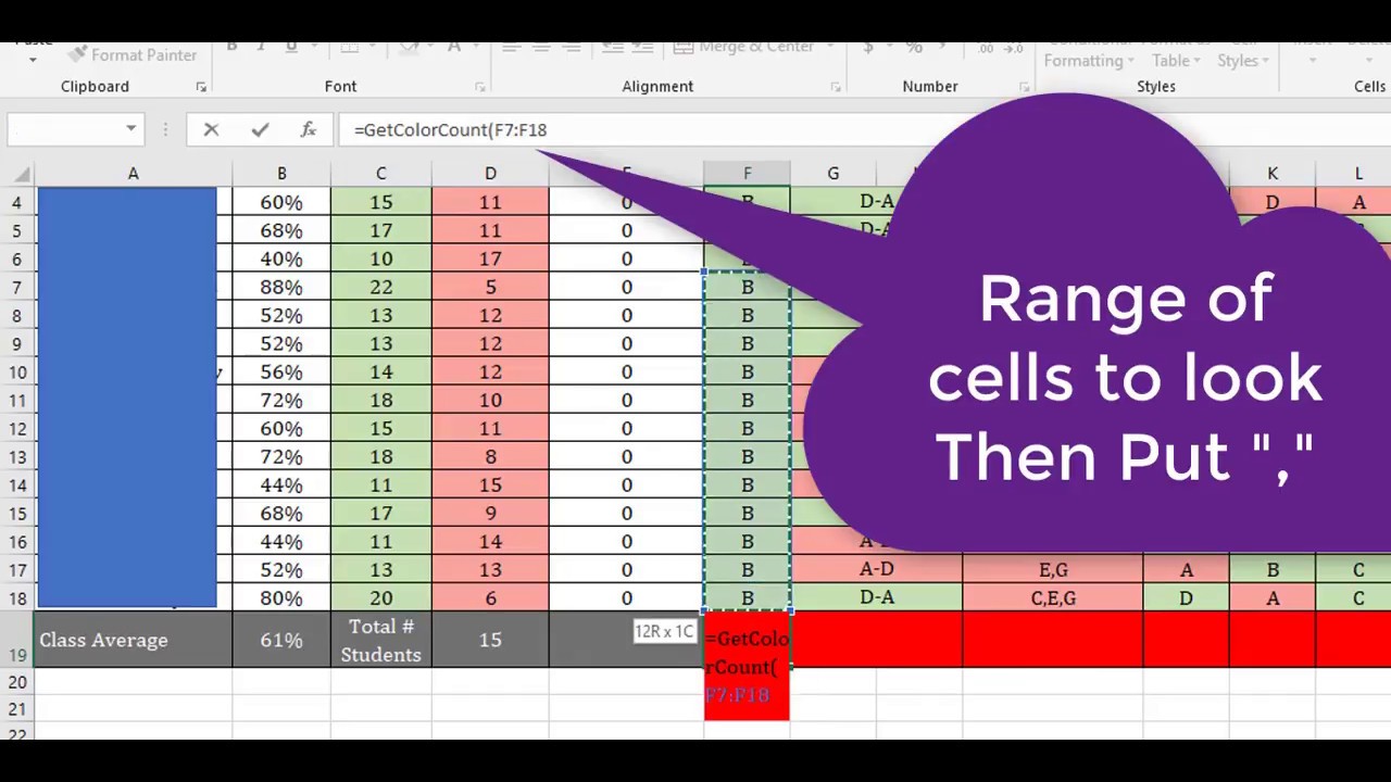
How To Count And Sum Cells By Color In Excel Youtube Images

How to Change MS Excel Cell Color Based on the Value of Another Cell

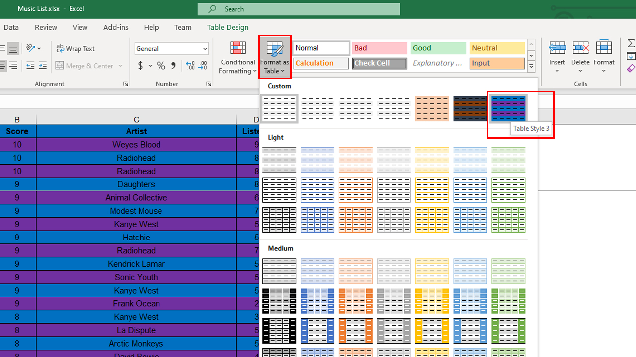
Type 'Dell' on the text box next to the second drop-down menu. Click the 'Format' button. On the 'Fill' tab of the 'Format Cells' dialog box, select red on the 'Background Color' palette and click OK. Click OK on the 'New Formatting Rule' dialog box. The cells containing 'Dell' will become red:

How to Color Cells in Excel Solve Your Tech

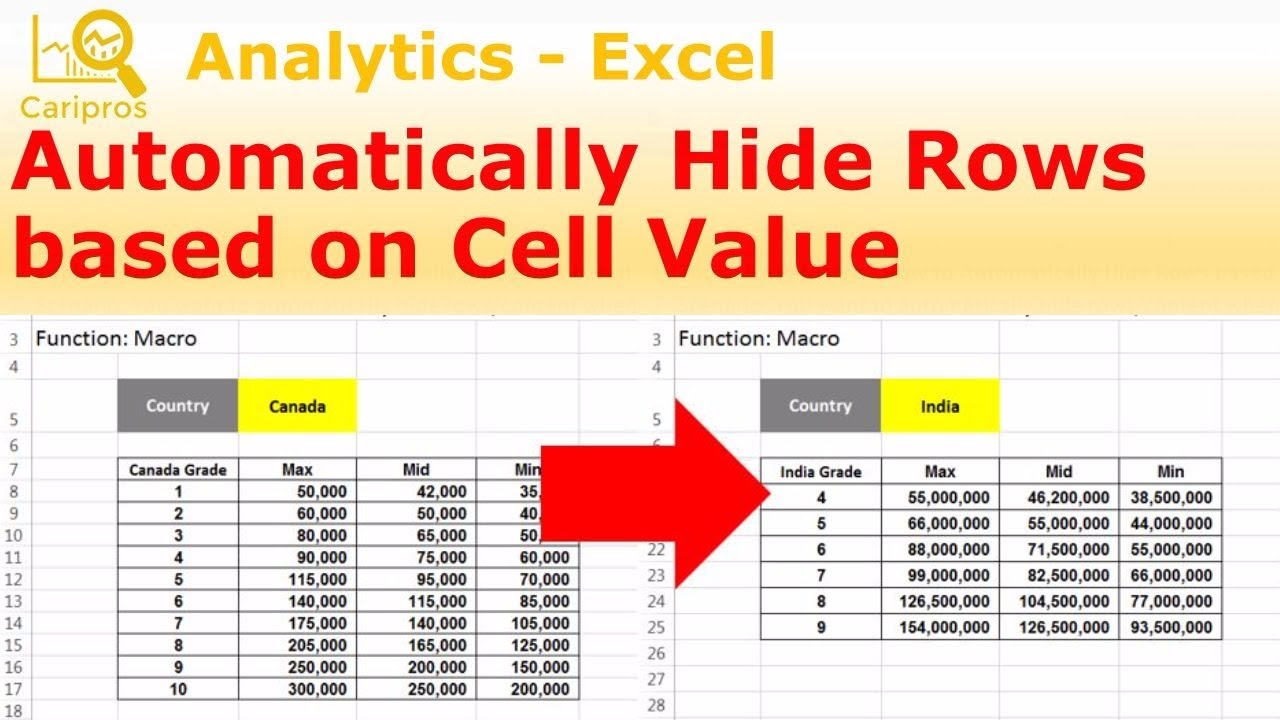
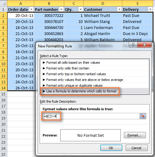
How to change a row color based on a number in a single cell. Say, you have a table of your company orders like this: You may want to shade the rows in different colors based on the cell value in the Qty. column to see the most important orders at a glance. This can be easily done using Excel Conditional Formatting.

Coloring Cell In Excel Based On Value Colette Cockrel

To color cells in Excel based on the value of another cell, follow these steps: Select the cells you want to format. Go to the "Home" tab and click "Conditional Formatting" > "New Rule." Select "Use a formula to determine which cells to format."

How to alternate cell colors in Microsoft Excel Laptop Mag

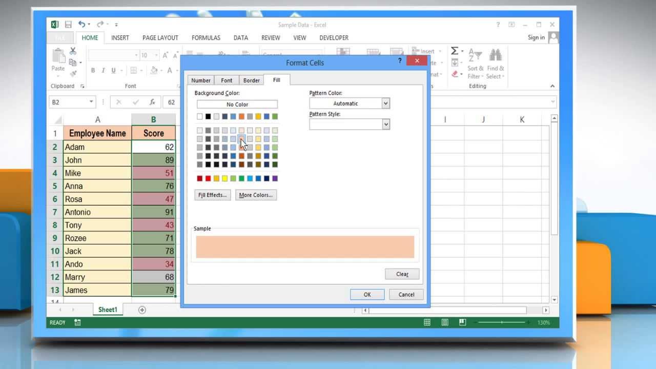
Select the cells that contain the numbers for which you want to change the font color. Click the Home tab. In the Styles group, click on Conditional Formatting. Hover the cursor over the option - 'Highlight Cell Rules'. Click on the 'Less than' option.

You Can Use The SUMIF Function In Excel To Sum Cells Based On

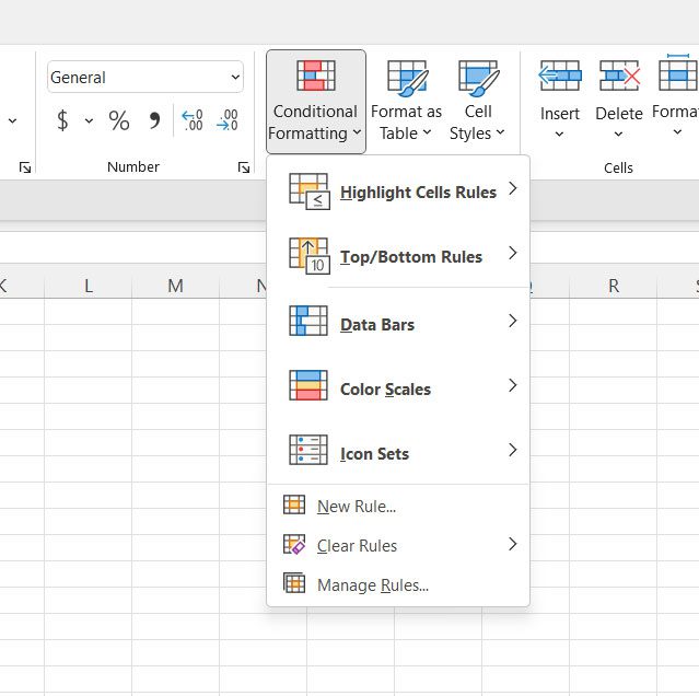
Step 1: Open your Excel spreadsheet and select the range of cells you want to apply the conditional formatting to. Step 2: Click on the 'Home' tab in the Excel ribbon at the top of the screen. Step 3: In the 'Styles' group, click on the 'Conditional Formatting' button. This will open a drop-down menu with various conditional formatting options.

How To Change Cell Color Based On Value In Excel 2023

On the Home tab, in the style section group, click on Conditional Formatting —-> New Rule. Note: Make sure the cell on which you want to apply conditional formatting is selected. Now select Use a formula to determine which cells to format, and in the box use the formula, D3>5, then select the formatting to fill the cell color to green. Now.

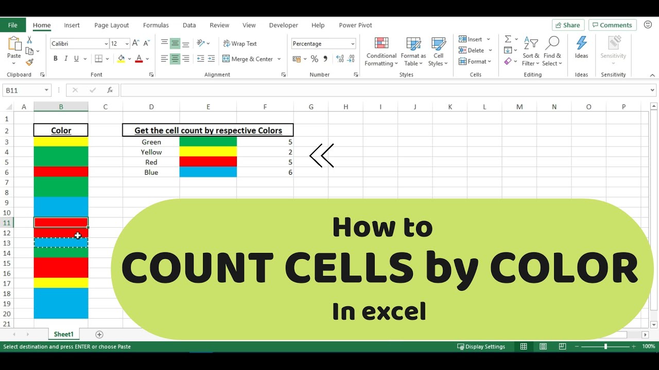
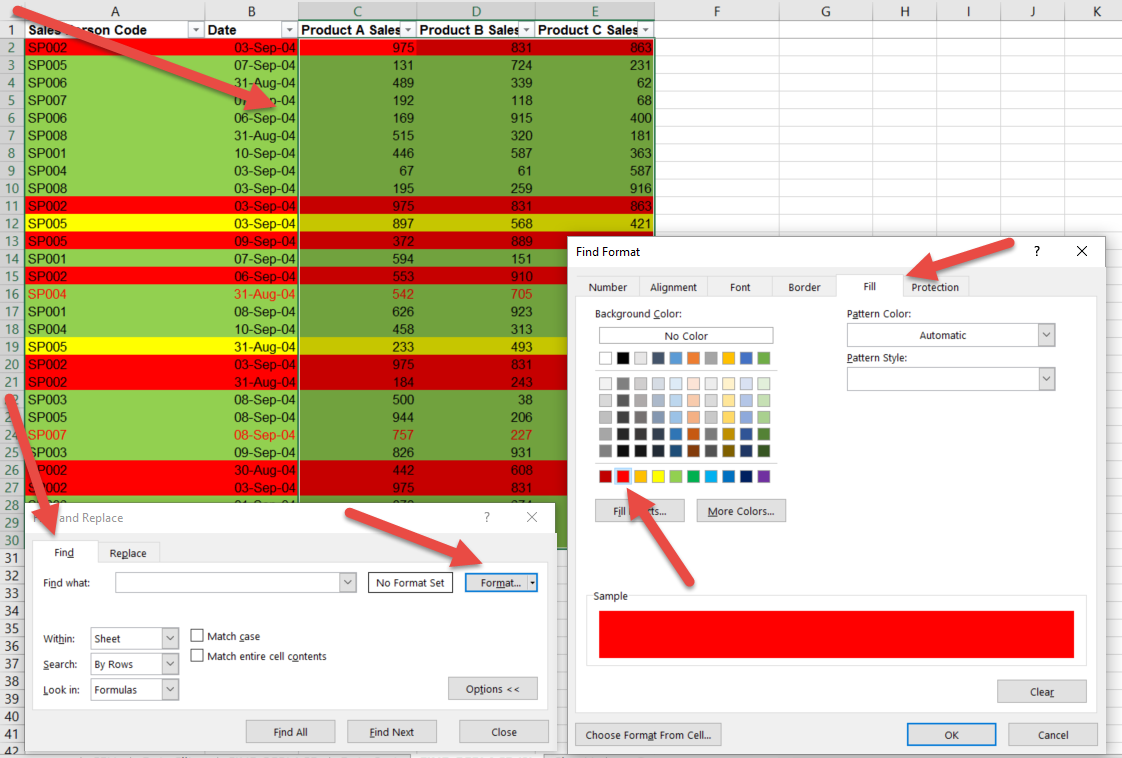
How to count cells based on color 🔴 Count colored cells in excel

In the Ribbon, select Home > Conditional Formatting > New Rule. Select Use a formula to determine which cells to format, and enter the formula: =E4="OverDue". Click on the Format button and select your desired formatting. Click OK, and then OK once again to return to the Conditional Formatting Rules Manager. Click Apply to apply the.

Excel Colour cells based around average of column for whole sheet

On the home tab, in the Styles subgroup, click on Conditional Formatting→New Rule. Now select Use a formula to determine which cells to format option, and in the box type the formula: D3>5; then select Format button to select green as the fill color. Keep in mind that we are changing the format of cell E3 based on cell D3 value, note that the.

how to color code cell in excel based on value Ms excel 2010 / how to

To apply conditional formatting based on a value in another cell, you can create a rule based on a simple formula. In the example shown, the formula used to apply conditional formatting to the range C5:G15 is:

Coloring Cell In Excel Based On Value Colette Cockrel

In Excel, you can change the cell color based on the value of another cell using conditional formatting. For example, you can highlight the names of sales reps in column A based on whether their sales are more than 450,000 or not (which is a value we have in cell D2).

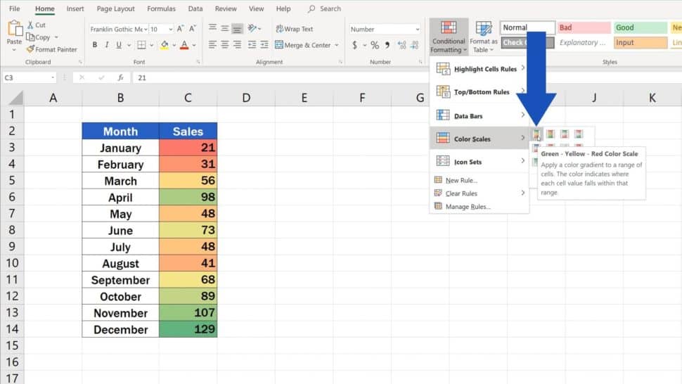
How to Use Color Scales in Excel (Conditional Formatting)

Custom Functions for Color-Related Calculations in Excel. When it comes to color-related calculations in Excel, custom functions can be a game-changer. These powerful tools allow you to extract information about cell colors, such as RGB values and color indexes, making it easier to analyze and manipulate data in Excel.

Excel Count Color Jajar Belajar

To use it, you create rules that determine the format of cells based on their values, such as the following monthly temperature data with cell colors tied to cell values. You can apply conditional formatting to a range of cells (either a selection or a named range), an Excel table, and in Excel for Windows, even a PivotTable report.

Counting Cells Based on Cell Color Excel YouTube

Select the cell and hover your mouse cursor in the lower portion of the selected range. A Quick Analysis Toolbar Icon will appear. Click on it. In the Formatting tab, select Greater Than. In the Greater Than tab, select the value above which the cells within the range will change color.

How to change Microsoft® Excel Cell Color based on cell value using the

How to use data bars to visually represent data in a cell. Select the range of cells where you want to apply data bars. Go to the "Home" tab and click on "Conditional Formatting." Choose "Data Bars" from the dropdown menu. Select a color option for the data bars that best suits your data representation needs. The length of the data bar in each.

Excel Change the row color based on cell value

Select the cells that you want to apply the formatting to by clicking and dragging through them. Then, head to the Styles section of the ribbon on the Home tab. Click "Conditional Formatting" and move your cursor to "Color Scales." You'll see all 12 options in the pop-out menu. As you hover your cursor over each one, you can see the arrangement.

How to Change Excel Cell Color Based on Cell Value Using The

Since we are interested in changing the color of empty cells, enter the formula =IsBlank (), then place the cursor between parentheses and click the Collapse Dialog button in the right-hand part of the window to select a range of cells, or you can type the range manually, e.g. =IsBlank(B2:H12) . Click the Format… button and choose the needed.